Summary

Time series momentum (TSMOM) is an investment strategy that involves buying assets whose prices are trending upward and shorting assets that have a downward trend. In 2012, Moskowitz, Ooi & Pedersen published Time Series Momentum¹. They analyzed a simple version of the strategy that buys assets with positive 12-month returns and shorts assets with negative 12-month returns. They found that the strategy had statistically significant outperformance in equity indexes, currencies, commodities, and bond futures from 1985 to 2009.

However, others have raised doubts. Huang, Li, Wang & Zhou (henceforth HLWZ) criticized the strategy in Time Series Momentum: Is It There? (2020)², concluding that the evidence for TSMOM is not statistically reliable.

Some of their criticisms have merit, but TSMOM remains an appealing strategy.

The abstract of Time Series Momentum: Is It There? reads:

Time series momentum (TSMOM³) refers to the predictability of the past 12-month return on the next one-month return and is the focus of several recent influential studies. This paper shows that asset-by-asset time series regressions reveal little evidence of TSMOM, both in- and out-of-sample. While the t-statistic in a pooled regression appears large, it is not statistically reliable as it is less than the critical values of parametric and nonparametric bootstraps. From an investment perspective, the TSMOM strategy is profitable, but its performance is virtually the same as that of a similar strategy that is based on historical sample mean and does not require predictability. Overall, the evidence on TSMOM is weak, particularly for the large cross section of assets.

To rephrase, HLWZ make two central arguments:

1. Moskowitz, Ooi & Pedersen (2012)¹ did a pooled regression and found a statistically significant correlation, but this methodology is flawed: it finds a strong correlation even when time series momentum cannot predict future prices.
2. TSMOM performed similarly to a strategy that simply buys assets with positive long-run historical returns and shorts assets with negative historical returns. The authors call this strategy Time Series History or TSH.

My responses to the two arguments:

1. I agree that a pooled regression is flawed. But a statistically significant correlation on a pooled regression is not what convinced me that TSMOM works. [More]
2. TSMOM and TSH indeed have similar(ish) historical returns. However:
   1. TSMOM’s positive performance cannot be explained by TSH alone. [More]
   2. TSMOM provided better diversification to an equity portfolio. [More]
   3. TSMOM has large unexplained returns when regressed onto a Fama-French factor model. [More]
   4. TSMOM still performed well on a much larger sample going back a century. [More]

TSMOM looks strong in the historical data. TSMOM probably survives fees and trading costs, but the evidence for that is less clear. [More]

Contents

• Summary
• Contents
• What is time series momentum, and what’s (allegedly) good about it?
• Responding to the critiques
  • The pooled regression critique
  • Is TSMOM just a fancy way of buying high-return assets?
  • Diversification benefits of TSMOM vs. TSH
  • HLWZ’s four-factor regression
  • The “more data” counterargument
• TSMOM: Yes, it’s there*
  • *Does TSMOM survive trading costs?
• Notes

What is time series momentum, and what’s (allegedly) good about it?

Time series momentum, also known as trendfollowing, works like this:

1. Get a big list of markets across equities, bonds, commodities, and currencies.
2. For each market, if it has been trending upward recently, buy it. If it’s been trending down, short it.

The exact definition of “trending upward” depends on implementation details. The simplest method is to look at the total return (minus the risk-free interest rate) over the last 12 months. If the total excess return is positive, that’s an uptrend; otherwise, it’s a downtrend. This definition is used by most research papers on TSMOM, including Moskowitz et al.¹ and their HLWZ².

The basic case for TSMOM (which HLWZ will argue against) is that historically it had positive returns with near-zero correlation to equities or bonds.

Table 1 compares the performance of the total US stock market versus an index of live trendfollowing funds (net of costs).⁴

	Sharpe Ratio	Return	Stdev	Skewness	Ulcer Index
US Equities	0.55	10.8%	15.5%	-0.8	13.5
Trend Index	0.40	7.5%	12.7%	0.3	7.3
50/50 Blend	0.72	9.8%	9.6%	-0.1	4.2

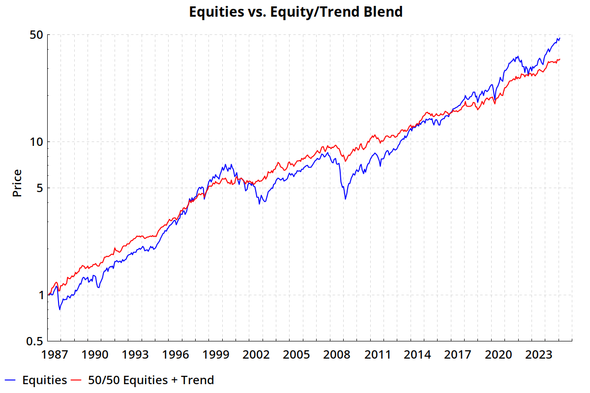
The trend index did not perform as well as US equities, but a 50/50 combination gave a better risk-adjusted return than either strategy alone.

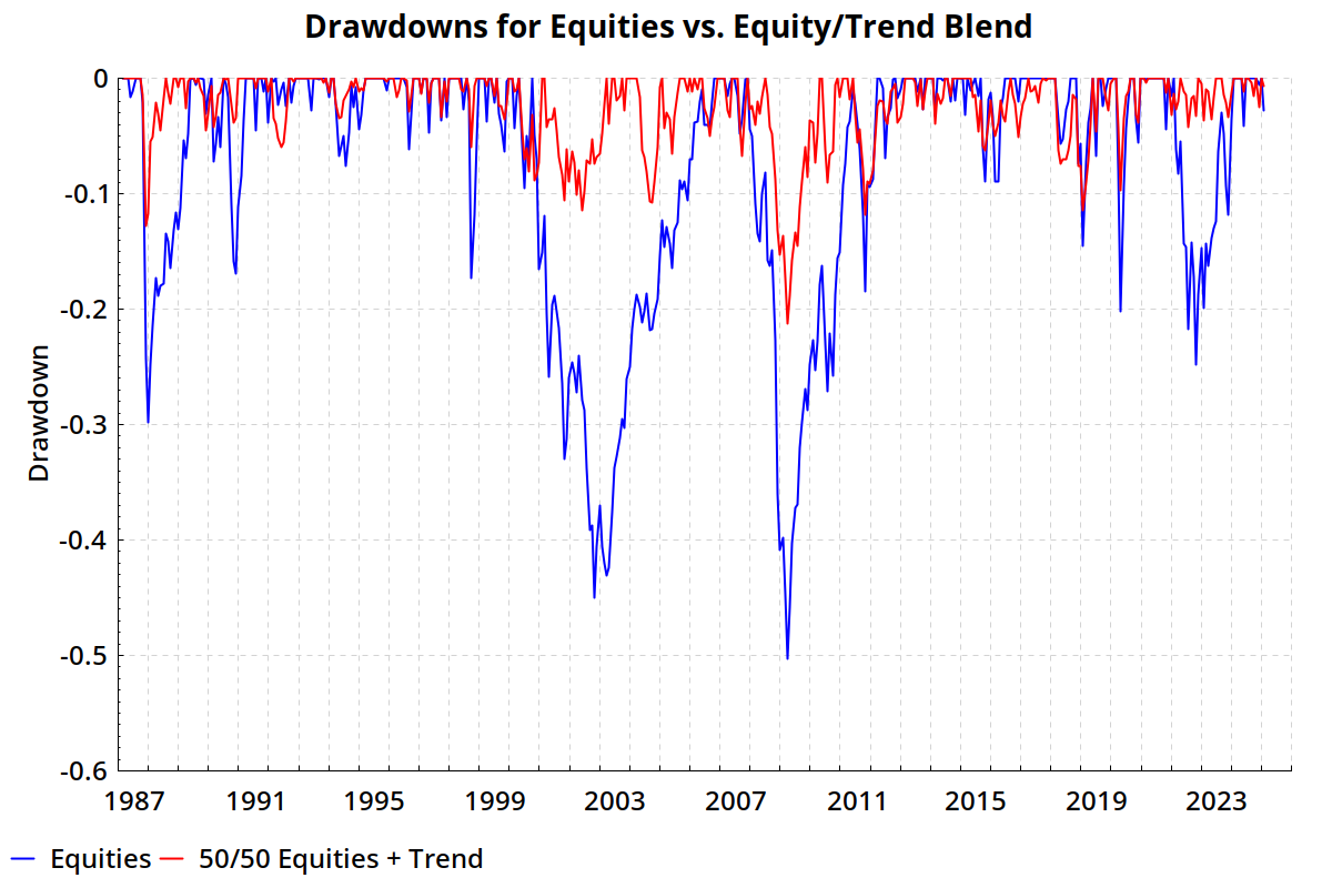
The ulcer index, a measurement of the frequency and severity of drawdowns, is a quantification of what we can see in the graph below: the 50/50 blend had a much softer downside than US equities.

For simplicity, I did not include bonds in this brief analysis, but looking at stocks + bonds + trend gives qualitatively similar results. For more, see Hurst, Ooi & Pedersen (2017)⁵, particularly the section “Performance During Crisis Periods” and Exhibits 6 and 7 (page 5–8).

Responding to the critiques

The pooled regression critique

Moskowitz, Ooi & Pedersen (2012)¹ wanted to determine if the past 12 months of returns of an asset could predict its future returns. Individual assets are too volatile to contain much signal; they got around this problem by pooling all assets together and running a single regression on all assets at once.

Huang, Li, Wang & Zhou (2020)² argued that the pooled regression technique is flawed because it creates a spurious correlation between past and future returns.

As an illustration, suppose we are studying time series momentum in the nation of Latveria. The country has just two tradable assets: Von Doom Industries equities (ticker symbol VDI) and Latverian Treasury bonds. Thanks to the unparalleled genius of Victor von Doom, the stock returns around 20% per year with only 5% volatility. The Latverian government is notoriously unreliable,⁶ however, and the bonds predictably lose 5% every year. (The government is reliable in its unreliability.)

If we run a pooled regression on Von Doom stocks + Latverian bonds, we will find strong evidence of time series momentum. A past 12-month return of 20% predicts a next-month return of 1.5% (= 20% annualized), and a –5% one-year return predicts a forward month return of –0.4%. The regression will show high predictability with a low p-value.

In actuality, there is no TSMOM in Latveria: returns are a random walk with no predictability. But pooling stocks and bonds together creates the appearance of predictability. High past returns provide evidence of high future returns, but only by telling you whether the asset you’re looking at is a stock or a bond.

HLWZ demonstrated this point with more rigorous statistics. The Latveria example captures the gist of their argument: a pooled regression makes it look like TSMOM can predict future returns, even when it can’t.⁷

I have no direct counter-argument. HLWZ are right to criticize the pooled regression method, and it is good to publish criticisms of incorrect arguments. But my enthusiasm for TSMOM as an investment strategy remains unperturbed by the pooled regression critique. The real question is not, is there a statistically significant covariance future returns and recent past returns of individual assets? The real question is, does TSMOM work?

HLWZ address this question as well, and they argue that the answer is no. Or rather, they argue that TSMOM works, but only by mimicking a simpler strategy that does not require time series predictability.

Is TSMOM just a fancy way of buying high-return assets?

The authors argue that TSMOM is not a genuine premium, but that it works by systematically buying assets with high average returns and shorting assets with low average returns.

Recall Latveria, with its stock that earns 20% per year and its bond that earns –5%. If you follow a TSMOM strategy on Latverian assets, you will find yourself holding stocks and shorting bonds, and you will earn 25% per year. Does that mean TSMOM works? No, because you could do just as well by simply buying stocks and shorting bonds. You don’t need to pay any attention to each asset’s past 12-month returns, and you don’t need to do any active trading.

Huang, Li, Wang & Zhou propose a strategy that they call Time Series History (TSH):

1. If an asset has a positive historical return, buy it.
2. If an asset has a negative historical return, short it.

In their Table 10, the authors show that TSMOM’s returns were not demonstrably better than those of TSH.

	annualized return8	t-stat	p-value	likelihood ratio
TSMOM	4.8%	4.73	< 0.001	53,000
TSH	3.0%	2.70	0.007	37

I calculated likelihood ratios as P(X=x|μ=x) / P(X=x|μ=0).⁹

The difference in returns between TSMOM and TSH was statistically insignificant (p = 0.19).

Does that mean TSMOM has no genuine signal, and it’s just an unnecessarily complicated way of buying assets with high returns?

No, because returns don’t tell the full story.

The question to ask is not, does TSMOM have a higher return than TSH? The question is, does TSMOM add value to a portfolio?

We saw before that real-world trendfollowing funds added diversification value to US equities even though they performed worse than equities on their own. However, my comparison from before was not statistically rigorous—how do we know that the diversification value wasn’t just luck?—so we need to do better than that.

We can ask two related questions:

1. Is TSMOM essentially just TSH?
2. For an investor who owns an equity index fund, does TSMOM add value? And does it add more value than TSH does?

As a first look at TSMOM vs. TSH, here’s a chart of their total returns 1986–2015. Notice the divergence in the circled areas:

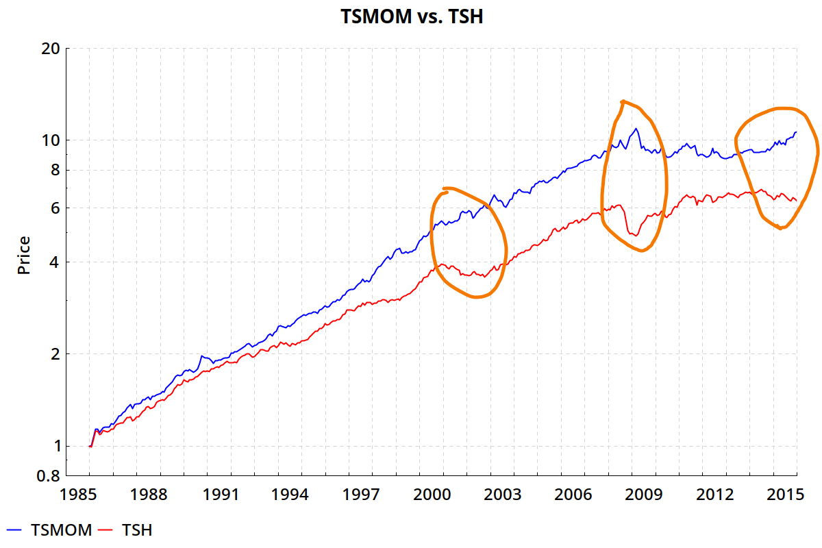
Those two lines don’t look the same. But the graph doesn’t tell us whether those divergences are statistically meaningful.

We can get a more reliable answer by running a linear regression of TSMOM with TSH as the independent variable. Does TSMOM have alpha relative to TSH?

HLWZ didn’t run that regression, but Guofu Zhou (the Z in HLWZ) helpfully published the code and data on his website,¹⁰ so I downloaded the data and ran the regression myself.

Here’s the result I got when regressing TSMOM onto TSH:¹¹

		t-stat	p-value	likelihood ratio
annual alpha (intercept)	4.17%	4.14	< 0.001	4,400
TSH (slope)	0.22	1.38	0.17	2.6
r2	0.04

An r² of 0.04 means that TSH can only explain 4% of the variance in TSMOM’s returns. An alpha of 4.17% means that, after subtracting the part of TSMOM that’s explained by TSH, TSMOM still had an annual return of 4.17%—and this alpha was highly statistically significant.

In fact, the TSH component of TSMOM was not significant: there is not good evidence that TSH can explain the returns of TSMOM at all.

As for the second question: do TSMOM and TSH add diversification benefits to an equity portfolio?

Diversification benefits of TSMOM vs. TSH

If we compare the historical drawdowns for TSMOM and TSH, TSMOM looks more painful to hold:

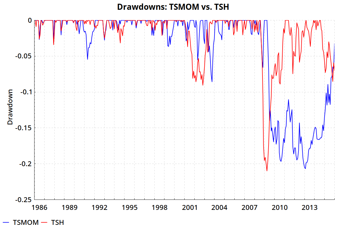
But notice when their biggest drawdowns occurred. The TSH portfolio lost 21% from July 2008 to March 2009. You know what else had a big drawdown that hit bottom in March 2009? The stock market. TSMOM’s biggest drawdown didn’t begin until March 2009, right when equities started recovering.

In isolation, TSMOM had more downside risk than TSH. But it looks much better as an addition to an equity portfolio:

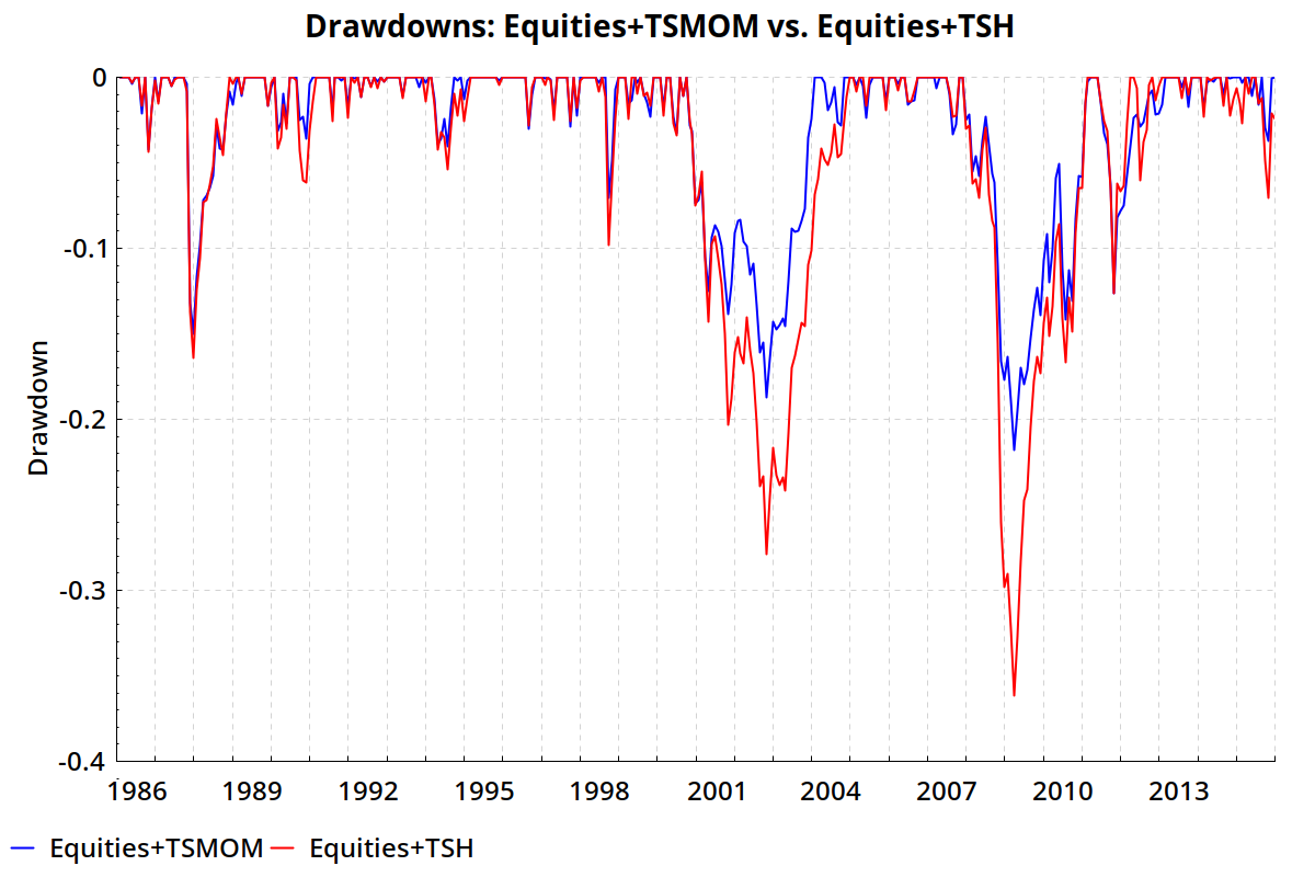
TSMOM provided a better cushion during the 2000–2003 and 2007–2009 bear markets.

For a more statistical perspective, I regressed TSMOM/TSH against US equities. From Table 4, we can see that:

• TSMOM was not explained at all by US equities, and it had statistically significant alpha.
• TSH was strongly explained by equities, and it had non-significant (although positive) alpha.

	TSMOM	t-stat	TSH	t-stat
annual alpha	5.06%***	(4.4)	1.50%	(1.7)
US equities	-0.03	(-1.3)	0.19***	(11.9)
r2	0.00		0.27

*, **, and *** indicate significance at the 0.05, 0.01, and 0.001 levels, respectively.

Bonus content: Summary statistics for TSMOM, TSH, and equity blends

	Sharpe Ratio	Return	Stdev	Ulcer Index
TSMOM	0.76	8.2%	6.2%	7.5
TSH	0.53	6.3%	5.6%	4.0
Equities+TSMOM	0.76	9.6%	8.2%	5.7
Equities+TSH	0.56	8.5%	9.5%	8.3

(Equity blends are 50% equities plus 50% the other strategy.)

TSMOM alone had a higher standard deviation and ulcer index than TSH, but Equities + TSMOM looks less risky than Equities + TSH.

HLWZ’s four-factor regression

Huang, Li, Wang & Zhou regressed TSMOM and TSH against the Fama-French four-factor model that includes the (global) equity beta, size, value, and momentum factors.

What's a Fama-French four-factor model?

In the beginning, there was the Efficient Market Hypothesis. The Capital Asset Pricing Model (CAPM) hypothesized that a stock’s risk is a function of its beta, which is a number describing how much it moves with the market. If a stock has a beta of 1, that means when the market goes up 1%, that stock also goes up 1%. A stock with a beta of 2 tends to move twice as much as the market. According to CAPM, the only way to reliably outperform the market is to increase the beta of your portfolio (which means you’re also increasing risk).

But then some research began posing challenges to CAPM. Banz (1981)¹² found that stocks of smaller companies tended to outperform stocks of large companies. Statman (1980)¹³ and Chan et al. (1991)¹⁴, among others, found that stocks with high ratios of book valuebook value = total assets – total liabilities to market value (B/M) tended to outperform stocks with low B/M ratios.

Fama & French (1992)¹⁵ proposed a new three-factor model as an alternative to CAPM. Instead of assessing the risk of a stock using beta alone, the three-factor model includes—you guessed it—three factors: beta, size, and B/M. Fama & French found that this model was much better than CAPM at explaining the variance in stocks’ returns.

Since then, other market anomalies have been proposed, and many researchers now prefer four-factor, five-factor, or even bigger models. Time Series Momentum: Is It There?² uses a four-factor model that includes beta, size, value, and momentum, where momentum is the tendency of stocks with high past 12-month returns to outperform stocks with low 12-month returns.

(If momentum sounds similar to TSMOM, that’s because it is. The key difference is that the momentum factor goes long stocks with high relative returns and shorts stocks with low relative returns, whereas TSMOM goes long or short based on an asset’s absolute return. For example, in a situation like the 2008 Global Financial Crisis where almost everything is down, the momentum factor shorts the stocks that are crashing the hardest while buying the stocks that only declined a little bit. Meanwhile, TSMOM simply shorts everything.)

To do a factor regression, take some investment strategy—in our case, TSMOM—and run a linear regression where the independent variables are the factors in your model: beta, size, value, and momentum. The regression tells you how much of your strategy’s performance can be explained by known factors. The regression’s intercept, or alpha, tells you how much of the performance can’t be explained.

If TSMOM has a large positive return but near-zero alpha, that means its performance can be explained by factors we already knew about; it’s not doing anything novel.

	TSMOM	(t-stat)	TSH	(t-stat)
annual alpha	1.81%	(1.94)	0.05%	(0.80)
beta	0.02	(0.61)	0.25***	(8.54)
size	-0.06	(-1.83)	0.11***	(3.70)
value	0.06	(1.01)	0.08**	(2.96)
momentum	0.60***	(9.99)	0.13**	(2.76)

*, **, and *** indicate significance at the 0.05, 0.01, and 0.001 levels, respectively.

The authors’ takeaway was that TSMOM does not work better than TSH. Indeed, the two strategies both had weak alphas. But there are some important differences, particularly on beta and momentum.

TSMOM had near-zero beta. HLWZ’s regression reinforces what we saw in the previous section: TSH is significantly related to equities, and TSMOM isn’t.

The most powerful factor for explaining TSMOM is momentum, sometimes called “cross-sectional momentum” to distinguish it from time series momentum. The momentum factor buys stocks with high relative returns and shorts stocks with low relative returns.

Cross-sectional momentum and time-series momentum are closely related to each other, so it’s unsurprising that the performance of TSMOM is heavily explained by momentum. This does not diminish the value of TSMOM as an addition to an equity portfolio; it only diminishes the appeal if you already invest in momentum. And when we look at an extended data set—which I will do in the next section—we can find good evidence that TSMOM adds value even to a portfolio that already includes momentum.

Even if TSMOM has only weak alpha on top of momentum, does that make TSMOM worse than momentum? Not necessarily. What happens if you switch TSMOM and momentum around, and regress momentum onto a four-factor model that includes market beta, size, value, and TSMOM?

Well, I did exactly that. I discovered that momentum had negative 0.37% annual alpha in its own regression, compared to the positive 1.46% of TSMOM that I got when I replicated HLWZ’s four-factor regression.¹⁶ Neither of these alphas were statistically significant, but this weakly suggests that TSMOM is, if anything, a stronger factor than momentum. This finding is consistent with prior research.

Prior research comparing momentum and TSMOM

Goyal & Jegadeesh (2015)¹⁷ examined momentum and TSMOM among individual equities for a variety of lookback periods (3 months, 6 months, 12 months, etc.). They found that TSMOM had significant alpha when regressed on momentum, but the reverse was not true. In fact, for most lookback periods, momentum had negative alpha (see the last two columns of their Table 2). The authors found that stock momentum could be rescued by combining it with a TSMOM overlay on the equity index,¹⁸ which is good news for stock momentum, but TSMOM still plays a central role in the rescued version of the strategy.

Moskowitz, Ooi & Pedersen (2012)¹ separately regressed multi-asset momentum and stock momentum onto TSMOM. They found negative alphas for both, although the alphas were not statistically significant in this case (t = -1.17 for multi-asset momentum and t = -0.93 for stock momentum; see Table 5, Panel B).

If we say TSMOM “isn’t there” because it’s largely explained by momentum, then it would be even more accurate to instead say momentum “isn’t there”.

Bonus content: Regression of TSMOM onto Fama-French global four factors plus TSH

		t-stat	likelihood ratio
annual alpha	1.57%	1.67	4.0
TSH	0.25*	2.50	22
beta	-0.04	-1.18	2.0
size	-0.09*	-2.53	24
value	0.04	0.70	1.3
momentum	0.56***	9.49	>1017

*, **, and *** indicate significance at the 0.05, 0.01, and 0.001 levels, respectively.

According to this regression:

• TSH partially explains the behavior of TSMOM. (TSH has more explanatory power when combined with the four-factor model than it did by itself (Table 3).¹⁹) However, it still comes nowhere close to fully explaining TSMOM.
• The other regression coefficients look qualitatively similar to when TSH wasn’t included. TSMOM has positive but non-significant alpha, near-zero beta, and a large exposure to the momentum factor.

The “more data” counterargument

What do you do when you find a non-statistically-significant positive alpha, and your data is underpowered to detect whether the alpha is real or spurious? You get more data.

In 2017, Hurst, Ooi & Pedersen published A Century of Evidence on Trend-Following Investing⁵ which extended the data from Moskowitz, Ooi & Pedersen (2012)¹ back to 1880. They found that a simulated TSMOM strategy—net of estimated trading costs and a 2-and-20 fee—earned a 7.3% return with a 9.7% standard deviation and zero correlation to US equities or bonds. The fact that TSMOM showed such strong results going back to 1880 is good evidence that the 1986–2015 findings were not a fluke.²⁰

However, Hurst et al.’s extended dataset does not counter the criticism that TSMOM might be explained by TSH or known factors like momentum.

Global Factor Premiums²¹ by Baltussen, Swinkels & van Vliet (2019) collected data going back to 1800 across equity, bond, commodity and currency markets to test six different factor premiums. Most importantly for our purposes, they included the momentum and TSMOM factors (they referred to the latter as “Trend”). Their paper did not provide evidence that’s directly relevant for our purposes, but they did provide replication data.¹⁰ I used that data to test if TSMOM has alpha when regressed on US equities²² plus the momentum and value factors.²³ I started the backtest in 1927 because that’s the start date of the Ken French data library’s time series on equities and interest rates.²⁴

I regressed TSMOM against five factors: equity beta, equity index value, equity index momentum, multi-asset value, and multi-asset momentum.²⁵

		t-stat	likelihood ratio
annual alpha	10.31%***	8.0	>1013
beta	0.00	0.3	1.03
Val^EQ	0.06	1.7	4
Mom^EQ	0.02	0.5	1.12
Val^MA	0.03	0.7	1.30
Mom^MA	0.57***	15.6	>1050
r2	0.27

^EQ indicates an equity index factor; ^MA indicates a multi-asset factor. *, **, and *** indicate significance at the 0.05, 0.01, and 0.001 levels, respectively.

From 1927 to 2016, TSMOM had alpha that can’t be explained by momentum.

Bonus content: Regression of TSMOM onto more factors, 1927–2016

As a more conservative test, I regressed TSMOM onto the combination of the Global Factor Premiums factors plus the Fama-French four-factor model:

		t-stat	likelihood ratio
annual alpha	8.74%***	6.8	>1010
FF beta	0.04*	2.0	7
FF size	-0.00	-0.1	1.00
FF value	0.08*	2.5	25
FF momentum	0.16***	6.7	>109
Val^EQ	0.06	1.6	3
Mom^EQ	-0.02	-0.4	1.09
Val^MA	0.03	0.8	1.40
Mom^MA	0.56***	15.3	>1048
r2	0.30

*, **, and *** indicate significance at the 0.05, 0.01, and 0.001 levels, respectively.

Adding the Fama-French factors gave the model a little more explanatory power but TSMOM still had highly significant alpha.

(It’s statistically questionable to regress against multiple similar factors because it risks overfitting, but it’s only questionable in that it can make alpha appear artificially small. In this case, alpha is still large and significant.)

As a more direct comparison to HLWZ, below is a regression of TSMOM onto the US four-factor model, 1927–2016. This is not a fair test because TSMOM is global, not US-only, but I am including it for completeness.

		t-stat	likelihood ratio
annual alpha	13.93%***	9.6	>1019
beta	0.05*	2.1	10
size	-0.01	-0.2	1.02
value	0.10**	3.0	84
momentum	0.23***	8.8	>1016
r2	0.07

TSMOM: Yes, it’s there*

*Gross of fees and trading costs.

In summary:

The pooled regression method of Moskowitz, Ooi & Pedersen (2012)¹ overstates TSMOM’s ability to predict future returns. However, TSMOM still has statistically strong historical results. HLWZ’s comparison of TSMOM to Time Series History (TSH) misses the mark: they correctly observe that both strategies had similar historical returns, but TSH mostly earned its returns via holding equities, while TSMOM had near-zero beta; and a regression of TSMOM onto TSH showed that TSH had little ability to explain why TSMOM earned positive returns. TSMOM was significantly explained by the momentum factor; conversely, however, the momentum factor had negative returns after controlling for TSMOM.

By extending the data back to 1927, the positive average return of TSMOM became highly statistically significant, even when regressing on the momentum factor.

The evidence strongly suggests that TSMOM is a real phenomenon: assets that are trending upward tend to outperform those that are trending down. But whether TSMOM survives trading costs is another question.

*Does TSMOM survive trading costs?

Compared with hypothetical backtests, live trendfollowing funds have notably worse performance. They have good returns in isolation, with near-zero correlation to equities, but their four-factor alphas are not statistically significant.

This is largely a data problem: we don’t have live fund performance going back far enough. It’s also a problem of cost: live funds perform worse than hypothetical backtests because they have management fees and trading costs. Even if there is genuine alpha, it will be smaller, and smaller numbers are statistically harder to detect.

To estimate costs, I compared an index of trendfollowing funds⁴ against AQR’s published Time Series Momentum dataset, which gives hypothetical returns to a TSMOM strategy like the one studied by HLWZ. Comparing the live index against AQR’s benchmark, the two had very similar volatility and drawdown characteristics, but the live funds underperformed by just under four percentage points per year (on average) from 1987 to 2024. That suggests an all-in cost of four percentage points per year.

AQR’s TSMOM benchmark had 4.95% annual alpha on a four-factor regression²⁶, which had a moderate t-statistic of 2.40 (p = 0.017). Due to fees and trading costs, the live trend index had 1.36% annual alpha, which was nowhere close to statistically significant (t = 0.60, p = 0.55). So we can’t confidently say that live funds survive trading costs.

However, this is not a fair comparison. As we saw before, TSMOM is heavily explained by the momentum factor; but the momentum factor is not free to trade, any more than TSMOM is.

A straightforward way to handle this is to subtract estimated trading costs from the momentum factor.²⁷ I did a four-factor regression with the added assumption that momentum costs the same amount to trade as TSMOM, as determined by the difference between the live trend index and AQR’s TSMOM index.

		t-stat	likelihood ratio
annual alpha	4.83%*	2.3	14
beta	-0.02	-0.4	1.09
size	-0.05	-0.9	1.51
value	0.08	1.4	3
momentum (net)	0.18***	4.5	21,000
r2	0.06

*, **, and *** indicate significance at the 0.05, 0.01, and 0.001 levels, respectively.

A t-stat of 2.3 is decent but not amazing. (Harvey et al. (2015)²⁸ propose that factors should need a t-stat of at least 3.0 to be considered significant.)

A second approach is to regress a live TSMOM fund against a live momentum fund. The downside of this approach is that most momentum funds have not existed for long. I ran a regression of AQR’s TSMOM fund (AQMIX) against AQR’s equity momentum fund (AMOMX) plus global equities (VT); AQMIX had 5.04% annual alpha, which was just barely statistically significant (t-stat = 1.97, p = 0.0499). But the fund history only goes back to 2010, so this test is underpowered to detect alpha (which we can see at a glance—5.04% is strong outperformance in practice, but it still only had p = 0.0499!).

Hurst, Ooi & Pedersen (2017)⁵ estimated trading costs for TSMOM going back to 1880, using the methods from Jones (2002)²⁹ plus live trading data. They extrapolated from the live data by assuming costs were twice as high before 2002 and six times as high before 1993. After subtracting estimated costs and a 2-and-20 fee, they found that TSMOM still had strong performance back to 1880—an annualized return of 7.3% with 9.7% volatility. Their methodology was reasonable; however, this is ultimately an estimate, not live performance.

I’m highly confident that TSMOM is a real phenomenon. But I’m only moderately confident that TSMOM can be exploited by investors.

Posted on Feb 04, 2026

Notes